Function: calc[CLTdiscr] - Central Limit Theorem for discrete distributions 

Calling Sequence:  

CLTdiscr
Parameters: 

f - generating function for a discrete distribution 

j - number of  variables in the initial sum of the random variables 

n - number of variables in the random sample 

Stand = true/false , true: distributions are standardized, false: distributions are not standardized 

Hist = true/false, true: plots histogram, : plots only the midpoint on the upper end of each rectangle of the histogram
K = false/k, if  k = positive integer the histogram with constant width is plotted independent of the choices of and . Otherwise, select false 

Description: 

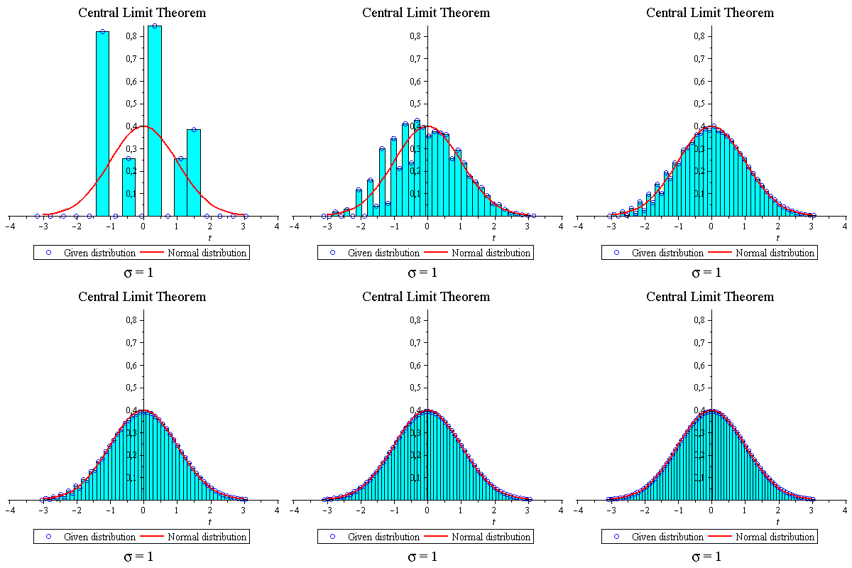
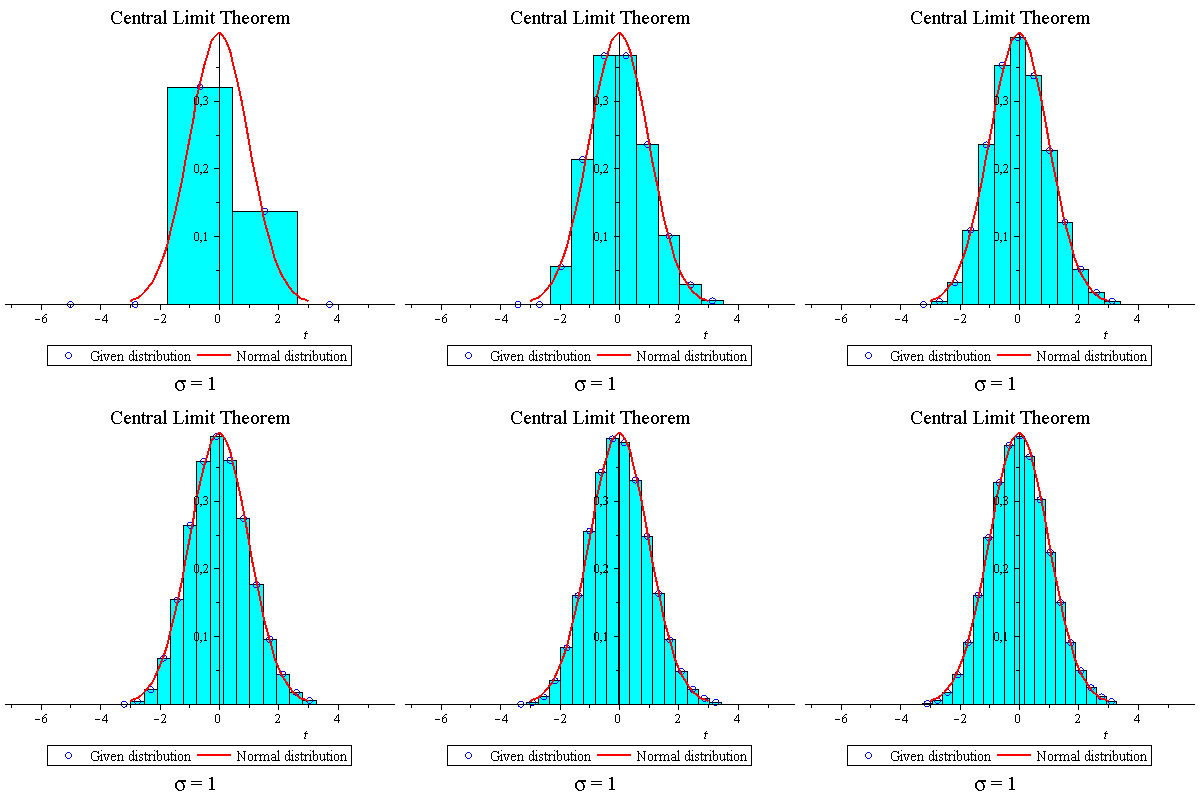
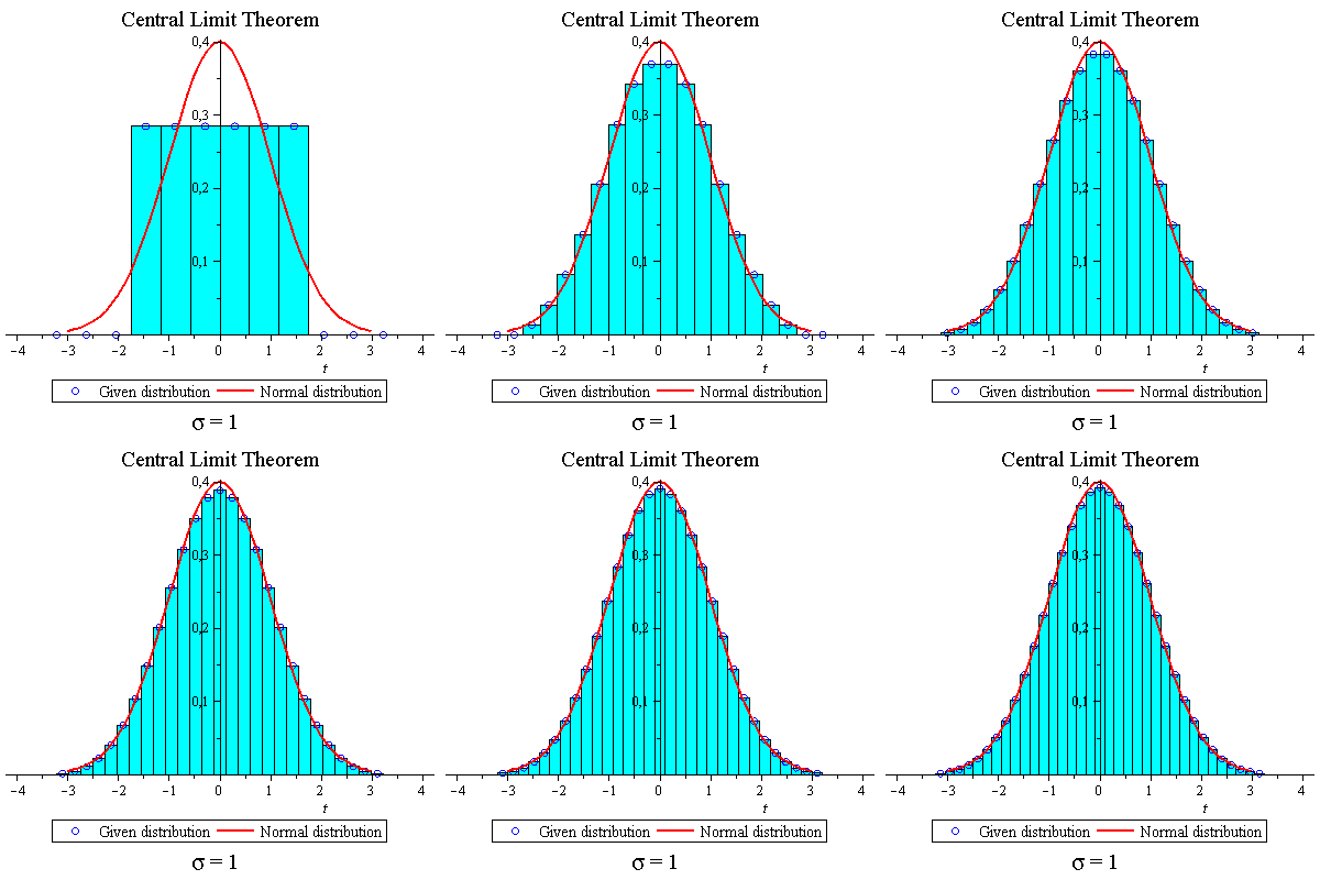
• CLTdiscr plots the distribution of the sum =  , = ,...,  as an animation. The plots are compared with the normal distribution with equal variance. All plots are located at the origin.

Examples: 

>	restart: with(calc):

 

>	f:=t->.32*t^(-3)+.1*t^(-1)+.33*t+.1*t^3+.15*t^4;

 

Some "messy" distribution  

>	CLTdiscr(f,1,20,true,true,false);

 

Skew binomial distribution 

>	f:=t->.7+.3*t;

 

>	CLTdiscr(f,1,40,true,true,false);

 

Throwing dice   

>	f:=t->1/6*t+1/6*t^2+1/6*t^3+1/6*t^4+1/6*t^5+1/6*t^6;

 

>	CLTdiscr(f,1,10,true,true,false);